Explainable AI for Pleural Effusion Detection
Final-year BSc dissertation · University of Northampton · Supervisor: Dr. Zenki
Detects pleural effusion in paired chest X-rays, explains the prediction with Grad-CAM++ heatmaps, and places the finding on a 3D lung model using both views.
- 87.24%Test accuracyTarget: 85%
- 94.11%AUC-ROCTarget: 0.93
- 82.01%SensitivityRecall on effusion cases
- 92.01%SpecificityCorrect on healthy cases
- 90.36%Precision
- 85.98%F1-score
Held-out test set of 3,761 CheXpert radiographs, split at patient level. One dataset, no external validation, no confidence intervals (single test partition).
Pleural effusion is fluid building up between the lung and the chest wall. This project takes a frontal and a lateral chest X-ray and does four things with them:
- Detects effusion with a single DenseNet-121 classifier trained on both view types.
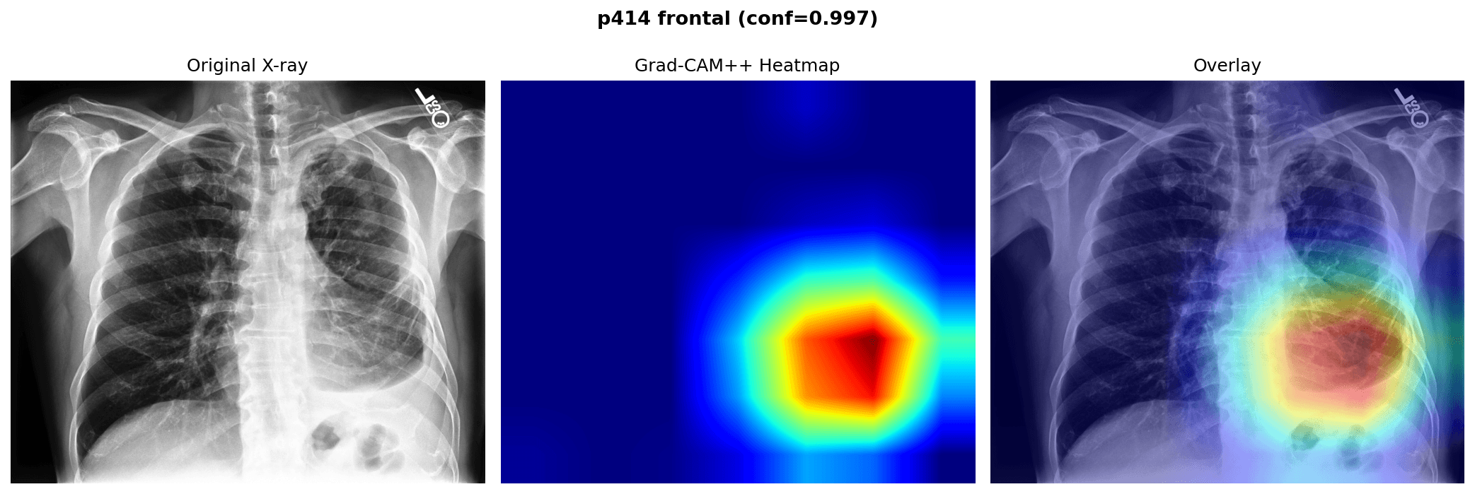
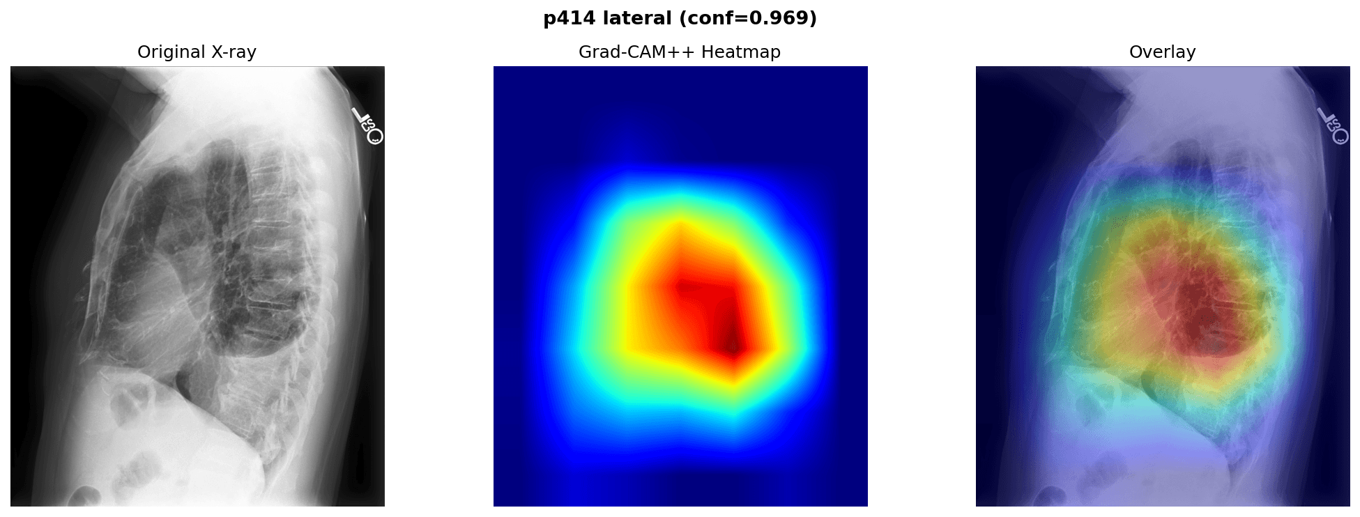
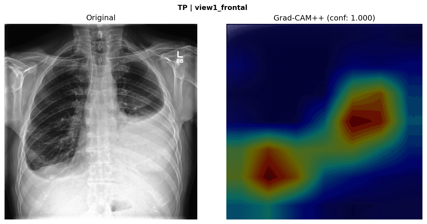
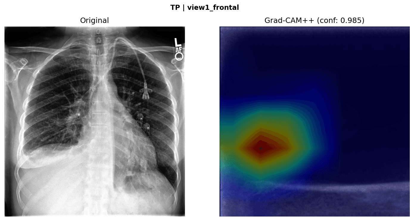
- Explains the prediction with Grad-CAM++ heatmaps on each view.
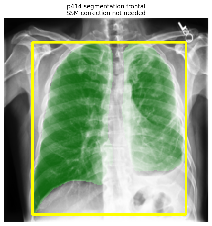
- Anchors the heatmaps to the patient's own lung boundaries, using lung segmentation corrected by a Statistical Shape Model.
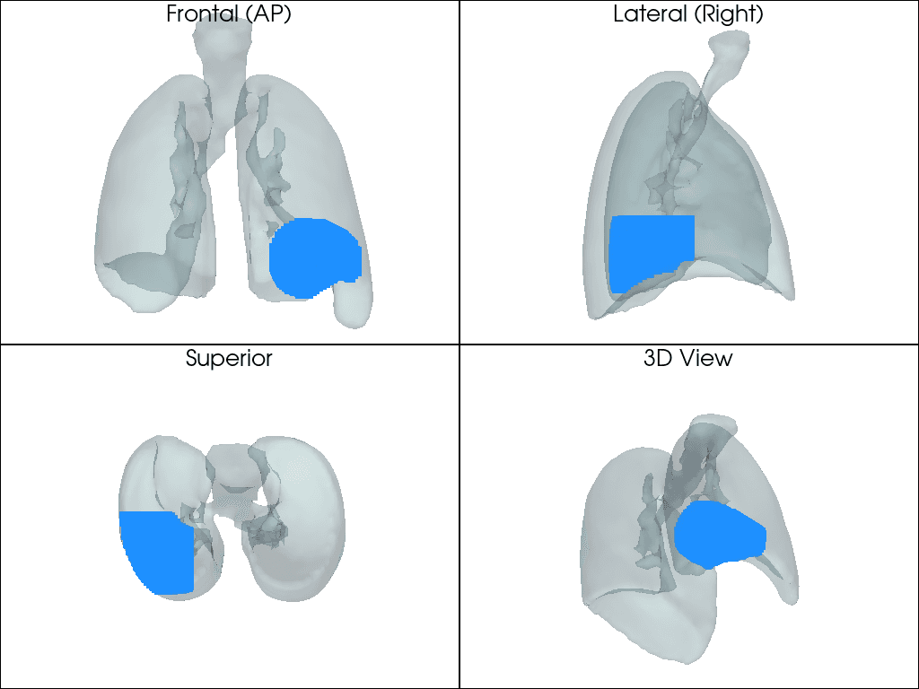
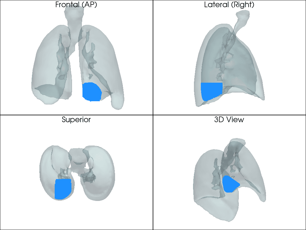
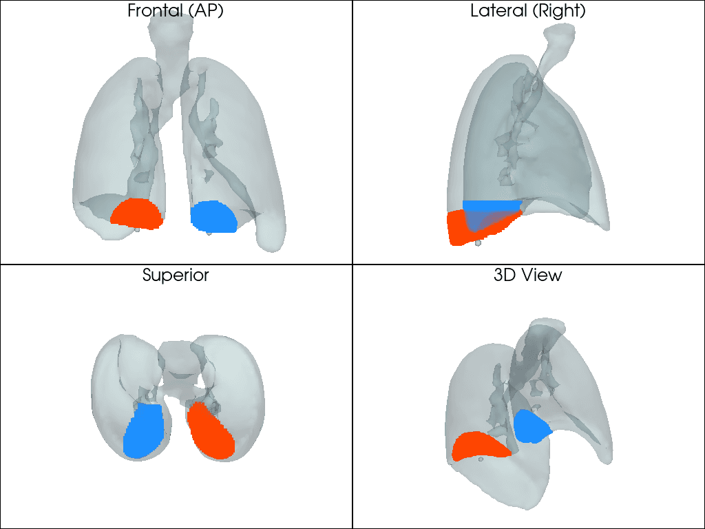
- Places the finding on a 3D lung model: the frontal view gives left/right and height, the lateral view gives front/back depth.
The goal is educational. It helps medical students connect a flat X-ray to where fluid actually sits in the chest. It is not a diagnostic tool.
Highlights
- 94.11% AUC-ROC and 87.24% accuracy on 3,761 held-out images, above the project targets of 0.93 and 85%.
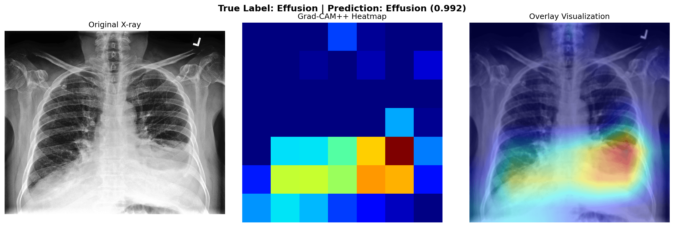
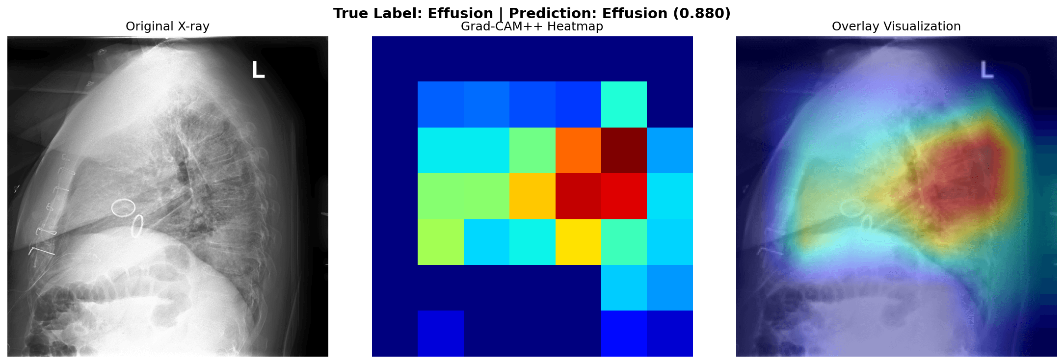
- 10 of 10 true-positive heatmaps activated in the lower lung fields and costophrenic angles in a 20-case qualitative check (not radiologist-validated).
- A shape-model fix for a failure I found in PSPNet: on effusion cases its lung mask stops at the fluid line. In the illustrated case the correction moved the lung base down by 31 px (13.8% of image height).
- A working dual-view to 3D pipeline with anatomically plausible placement on the four cases shown. There is no quantitative localisation error because no ground truth exists.
My role
I was the sole author of this dissertation project, supervised by Dr. Zenki. I chose the problem and scope, prepared the CheXpert data, trained and evaluated the classifier, and designed the lung-segmentation correction and the dual-view mapping onto a 3D lung model. My supervisor suggested replacing my original two-encoder design with a single unified model, which I adopted. Implementation code was developed with AI coding assistance; the design decisions, experiments and evaluation described here are mine.
The problem
Pleural effusion is one of the most common chest conditions and can point to heart failure, pneumonia, cancer or pulmonary embolism. A chest X-ray is the first-line test, but reading one means mentally rebuilding a 3D chest from a flat 2D projection. That is hard for students, and it matters here because the key sign, blunting of the costophrenic angle (the lower corner where lung meets diaphragm), is inherently spatial.
Three gaps motivated the project:
- Black-box models. Deep-learning classifiers detect pathology but rarely show why. Without an explanation you cannot tell whether a model is looking at the lung or at something irrelevant, such as a pacemaker.
- Frontal-only research. Most published work uses frontal X-rays only, although radiologists routinely use a lateral view too, and the lateral view is more sensitive to fluid settling at the back of the chest.
- No cheap route from 2D to 3D. Generating 3D anatomy from X-rays with generative models is computationally heavy and can invent anatomical detail that is not there, which is a poor fit for teaching.
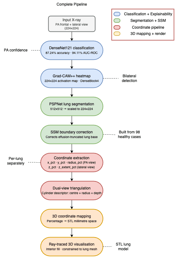
Approach: a five-stage pipeline
| Stage | Question it answers | Method |
|---|---|---|
| 1. Classify | Is there an effusion? | One DenseNet-121 (TorchXRayVision medical weights) for both views |
| 2. Explain | Where did the model look? | Grad-CAM++ on the last dense block |
| 3. Segment | Where are this patient's lungs? | PSPNet, with a Statistical Shape Model correcting the lung base |
| 4. Triangulate | Where is the finding in the chest? | x and y from the frontal view, depth z from the lateral view, as percentages of the lung box |
| 5. Render | What does that look like in 3D? | Ray-traced point cloud inside an STL lung mesh (PyVista) |
Two principles kept the scope realistic:
- No generative reconstruction. It risks producing plausible but non-existent anatomy, which is unsuitable for teaching.
- Use what clinics already acquire. Paired frontal and lateral radiographs are standard practice and contain enough orthogonal information to triangulate onto a reference 3D model, with no extra data collection.
The system is written in Python 3.10 with PyTorch. TorchXRayVision supplied the pretrained DenseNet-121 and PSPNet, and PyVista handled the 3D mesh and ray-tracing. I developed on a MacBook M3 Max and trained on the university's NVIDIA GPU infrastructure, using device-agnostic PyTorch code (CUDA, MPS or CPU).
Data and preparation
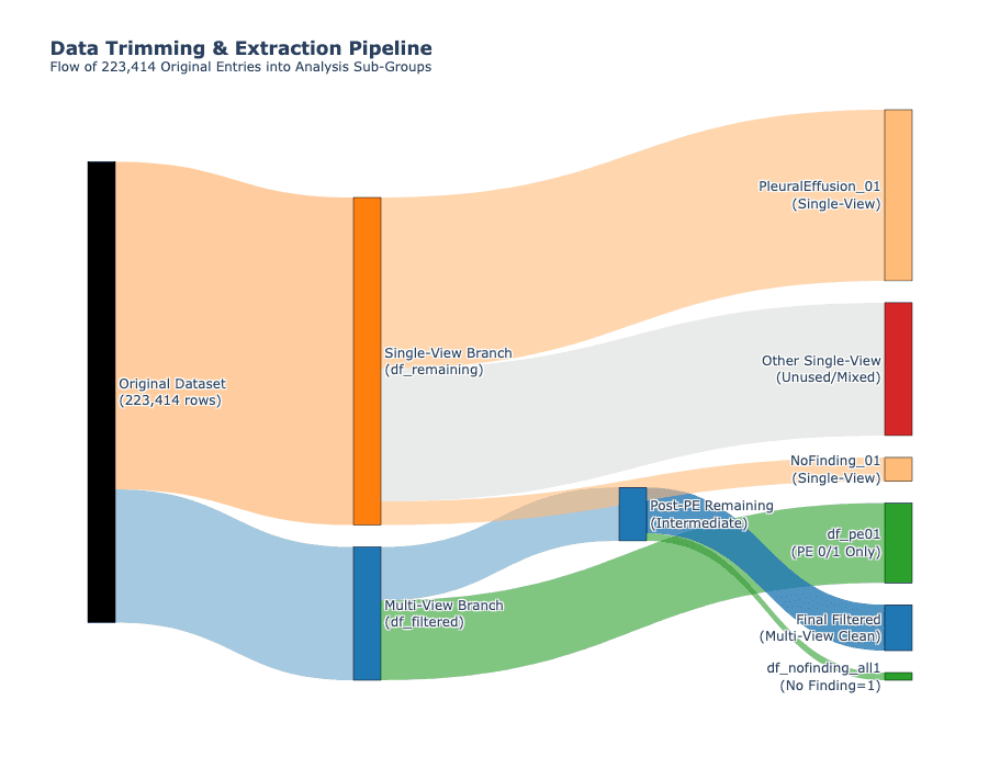
I used Stanford's CheXpert dataset: 223,414 entries from 65,240 patients. I chose it because it is the largest public chest-radiograph collection with paired frontal and lateral views for most patients, it labels uncertainty explicitly, and it is the standard benchmark for pleural effusion. I compared it with NIH ChestX-ray14 and MIMIC-CXR first.
Key preparation decisions:
- Uncertain labels removed. CheXpert marks findings a radiologist could not call as -1. Treating those as positive or negative would add label noise, so I excluded every case with an uncertain effusion label and kept only confirmed positives and negatives.
- Two subsets, handled separately. Multi-view studies (frontal and lateral, essential for triangulation) and single-view studies (frontal only) went down separate branches, so single-view data was not simply thrown away.
- Patient-level split. All images from one patient sit in exactly one of train, validation or test, which prevents patient-specific features leaking into the test score.
- Class balance. About 55% of the combined training data was effusion-positive.
| Split | Images | Strategy |
|---|---|---|
| Training | 29,000 | Patient-level |
| Validation | 3,600 | Patient-level |
| Test | 3,761 | Patient-level, held out |
| Total | 36,361 | No patient overlap |
Final dataset split used for model training and evaluation. Radiographs are single-channel grayscale at 224×224.
The classifier: one DenseNet-121 for both views

Why DenseNet-121. Dense connections keep low-level detail such as bone edges and diaphragm outlines available throughout the network. It is compact (about 8 million parameters versus roughly 25 million for ResNet-50), which lowers overfitting risk and speeds inference, and its convolutional feature maps suit Grad-CAM++. I considered a Vision Transformer, but ViTs need far more data without heavy pretraining and fit gradient-based explanation less naturally. The weights come from TorchXRayVision, pretrained on large medical-imaging collections, a stronger starting point than generic ImageNet weights.
One model, not two. My first design used a separate encoder for each view plus a fusion layer. My supervisor asked why two encoders were needed, and we agreed a single network trained on both view types would be simpler and likely just as effective. Each image is treated as an independent sample, so the model learns what the views share (fluid opacity, costophrenic angle blunting) rather than view-specific features. Earlier work (Hashir et al., 2020) found that adding lateral views helps whatever the fusion strategy.
Two-phase fine-tuning
| Phase 1 | Phase 2 | |
|---|---|---|
| What trains | New classifier head only (backbone frozen) | DenseBlock4 and the head |
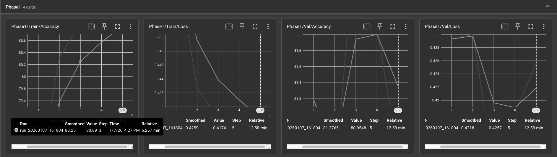
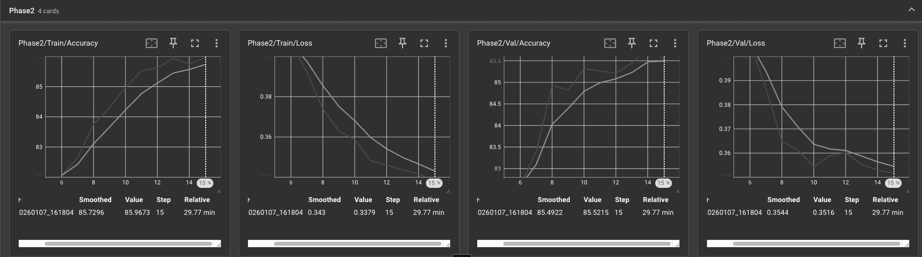
| Epochs | 5 | 9 more; early stopping (patience 3) ended training at epoch 14 |
| Optimiser and learning rate | Adam, 1e-3 (weight decay 1e-4), BCEWithLogitsLoss | 5e-5 for the backbone, 1e-4 for the head |
| Why | Adapt the head without disturbing the pretrained medical features | Let the deepest features specialise to effusion without wrecking earlier layers |
Training augmentation was random horizontal flips, rotation within ±10° and brightness/contrast changes within ±20%, to mimic natural variation in positioning and acquisition. No augmentation was applied at validation or test time.
Explainability: Grad-CAM++ heatmaps
Standard Grad-CAM averages gradients over each channel, so in bilateral effusion the stronger side can dominate the heatmap. Grad-CAM++ weights pixels using higher-order gradient information, so several regions can light up independently, which matters when fluid is on both sides. I hook DenseBlock4, which holds the most semantic features while keeping enough spatial resolution for a useful map, upsample the result to 224×224 with bilinear interpolation and normalise it to 0–1.
For coordinate extraction, the heatmap is thresholded at a fraction of its peak and the surviving region gives the position and size of the finding.
Choosing the activation threshold
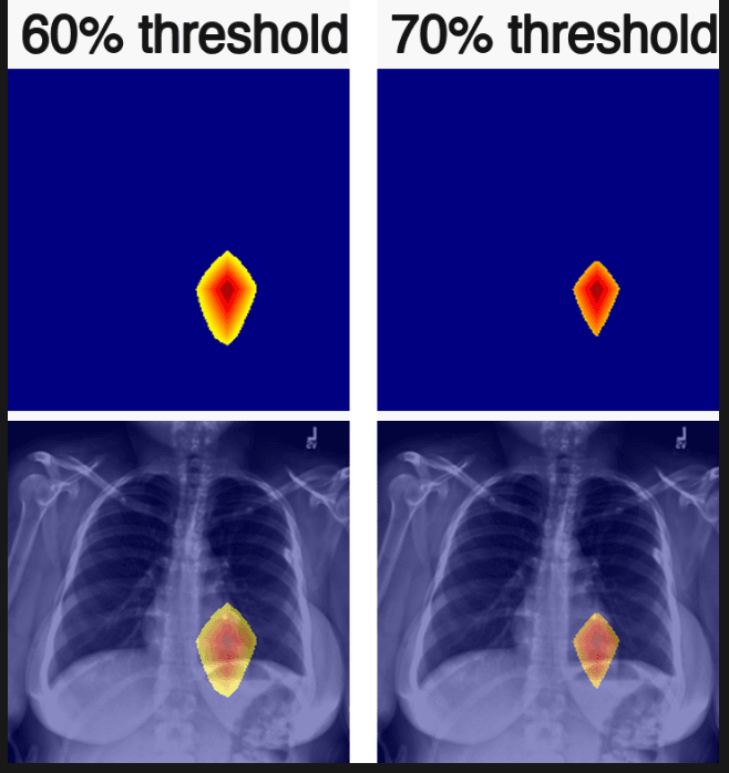
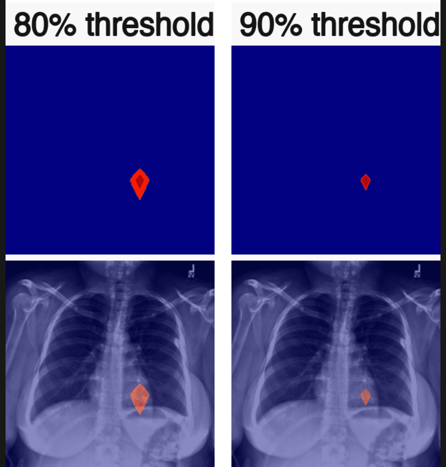
I compared 60%, 70%, 80% and 90% of the heatmap maximum on held-out cases and chose 80%.
| Threshold | What I observed |
|---|---|
| 60% | Broad region including low-confidence surrounding activation; diffuse, so the centroid is less precise |
| 70% | Tighter, but still includes transitional areas around the main peak |
| 80% (chosen) | Compact, stable region centred on the main peak; a reliable centroid and bounding box |
| 90% | Only a few pixels; the centroid is sensitive to noise and can suppress relevant activation in lower-confidence cases |
Lung segmentation and the shape-model fix
A raw heatmap coordinate lives in 224×224 image space. To map it onto a generic 3D lung, I need it relative to each patient's own lung boundaries, so that “near the base of the lung” means the same thing whatever the image scale or the patient's position. That needs a lung mask.
Attempt 1: intensity thresholding (rejected)
Lungs are dark on an X-ray, so I first tried a brightness threshold. It labelled about 93% of the image as lung. In a radiograph every structure is projected onto the same plane, so no single threshold can separate them. Deep-learning segmentation was required.
Attempt 2: PSPNet (good, but it fails on effusion)
TorchXRayVision's PSPNet separates both lungs cleanly on frontal views. I run it at its native 512×512 resolution (224×224 gave noticeably worse masks) and rescale boundaries by 224/512, with the mask thresholded at 0.3. Testing on effusion-positive cases exposed two problems:
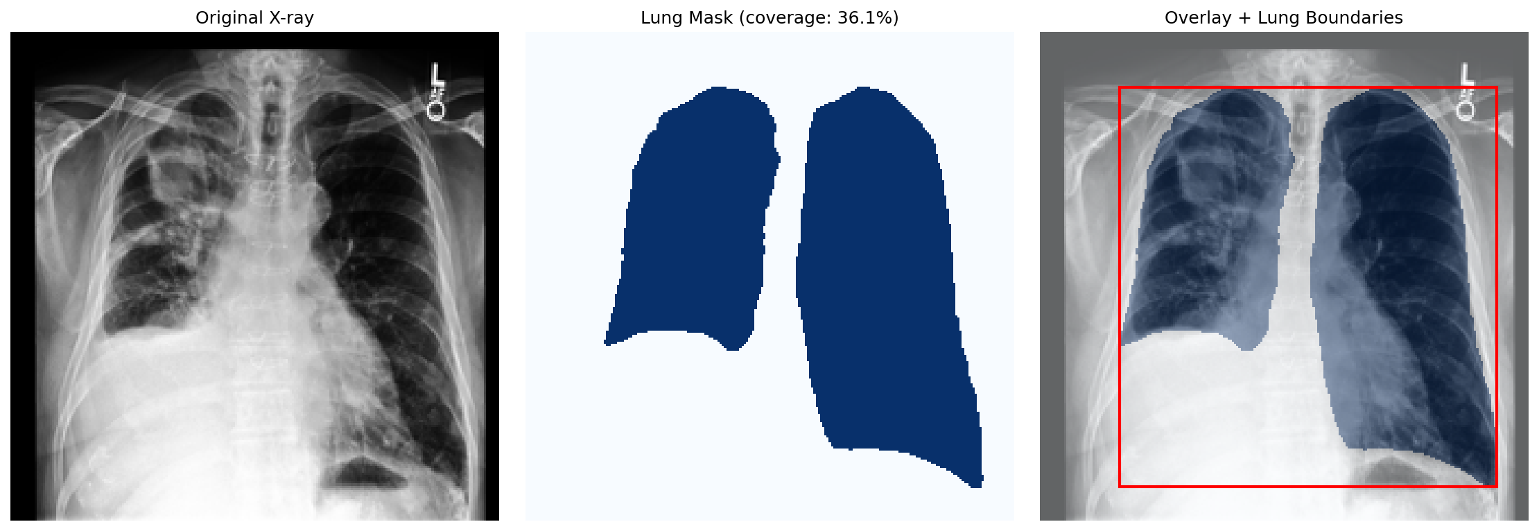
- Effusion truncation. PSPNet was trained to segment air-filled lung. Fluid is radio-opaque, so it is (correctly) “not lung”, and the mask stops at the fluid line instead of the true lung base. The Grad-CAM++ peak at the costophrenic angle then falls outside the mask, which makes normalising against it meaningless.
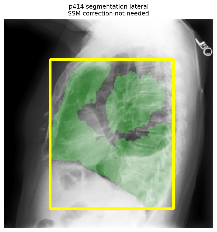
- Lateral fragmentation. PSPNet was trained mostly on frontal images, so lateral views come back as disconnected blobs that inflate the bounding box used for depth.
The fix: a Statistical Shape Model (SSM)
Even in severe effusion PSPNet reliably finds the upper part of the lungs, because the apex stays air-filled. The SSM uses that reliable top boundary to anchor the mean shape of a healthy lung, then predicts where the base should be if there were no effusion. I rejected the simpler idea of expanding every mask downwards by a fixed 15%: displacement varies with severity, and a fixed expansion would distort healthy cases.
Building the model. I sampled 100 confirmed-healthy frontal cases (random seed 42); 98 gave valid lung contours. Each contour was resampled to 80 landmarks (40 per lung, a 160-value shape vector) and aligned with Generalised Procrustes Analysis, which converged in 4 iterations. PCA on the aligned shapes gave 5 modes explaining about 80% of shape variation; the mean shape is the reference.
Using it. At inference the mean shape is scaled to the detected lung width and anchored at the detected top. The predicted lung base is compared with PSPNet's. If they differ by more than 8% of image height, the SSM boundary replaces PSPNet's. The correction is adaptive (healthy cases are left alone) and adds no extra neural-network inference.
Lateral views. I keep only the two largest connected components above 500 px² and discard the rest. The SSM is deliberately not applied, because its mean shape comes from frontal landmarks and is geometrically invalid for a lateral projection.
From heatmap to a position in 3D
From a point to a cylinder
My first plan was to represent an effusion as a single (x, y, z) point. A point says nothing about extent: a small effusion and a large bilateral one with the same centre would look identical. Each effusion is instead a cylinder, with a radius (lateral spread in the frontal view), a vertical extent, and an anteroposterior depth taken from the lateral heatmap.
Dual-view decomposition
The frontal view gives the horizontal (x) and vertical (y) position. The lateral view gives the depth (z), whether the fluid sits towards the front or the back. That is the only way, from plain radiographs, to confirm the posterior pooling expected in an upright patient. Left and right lungs are separated with connected-component analysis (assigned by centroid, following radiological convention), and every value is a percentage of that lung's SSM-corrected box. That makes the numbers patient-independent and directly mappable onto one generic model.
| Value | From | Meaning |
|---|---|---|
| x_pct | Frontal | Horizontal centre within the lung |
| y_pct | Frontal | Vertical centre; close to 1.0 means the lung base |
| radius_pct | Frontal | Radius of the equivalent circle (lateral spread) |
| y_top_pct, y_bot_pct | Frontal | Vertical extent of the cylinder |
| z_pct | Lateral | Anteroposterior depth position |
| z_extent_pct | Lateral | Anteroposterior length |
Percentages to millimetres
Z_world = Z_max - y_pct × (Z_max - Z_min)
Y_world = Y_max - z_pct × (Y_max - Y_min)The 3D lung model and the ray-traced fill
I evaluated Embodi3D, the NIH 3D Print Exchange and BodyParts3D, and chose a combined bilateral lung mesh from Embodi3D (derived from an XCAT phantom inhale model). Separate left and right meshes were rejected because aligning two coordinate systems complicates ray-tracing. I calibrated the mesh bounds once, in a prototype phase, by ray-scanning along each axis, so rendering uses fixed constants and is fast and reproducible.
A floating cylinder would not follow the concave lung surface and would look anatomically wrong. Instead I sample a 30×30 grid across the cylinder's cross-section and cast a ray through the mesh for each position. The entry and exit points from PyVista's ray_trace() are clipped to the cylinder's anteroposterior extent, so only points inside the lung volume are drawn and the highlight is always anatomically bounded.
Results
Classification
| Metric | Value |
|---|---|
| Test accuracy | 87.24% |
| AUC-ROC | 94.11% |
| Precision | 90.36% |
| Recall (sensitivity) | 82.01% |
| Specificity | 92.01% |
| F1-score | 85.98% |
| Validation accuracy | 85.83% |
| Training loss (best) | 0.3416 |
Held-out CheXpert test set (3,761 images). A single partition was used, so no confidence intervals were computed.
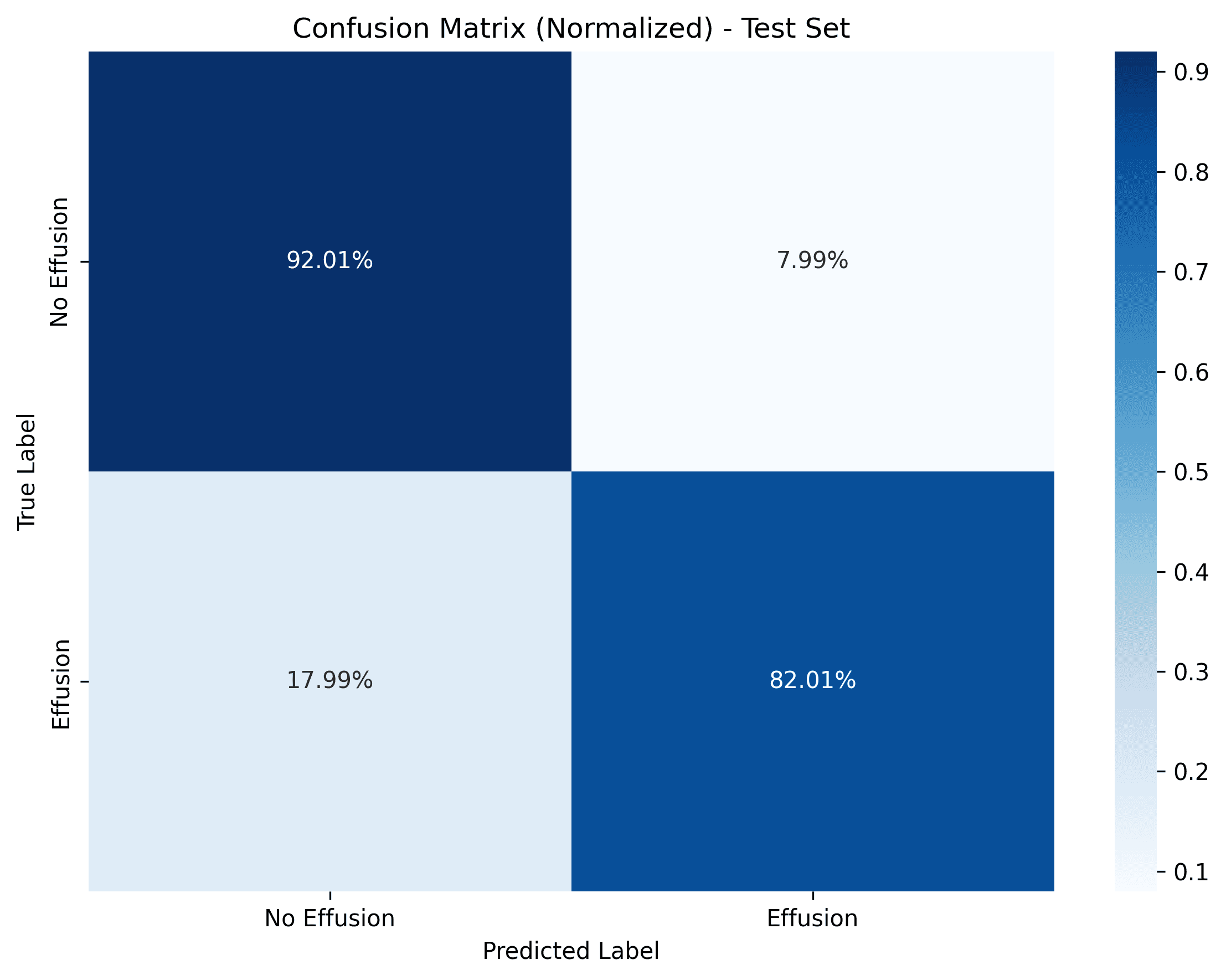
| True class | Predicted: effusion | Predicted: no effusion | Total |
|---|---|---|---|
| Effusion | 1,472 (TP) | 323 (FN) | 1,795 |
| No effusion | 157 (FP) | 1,809 (TN) | 1,966 |
The same matrix as raw counts.
Reading the numbers. An AUC-ROC of 0.941 means the model ranks a random effusion case above a random healthy case about 94% of the time. Specificity (92.0%) is higher than sensitivity (82.0%), so the model misses more effusions (323) than it falsely flags (157). For a screening tool a missed effusion is the more serious error. The decision threshold could be tuned or the data rebalanced, but I did not, because this is an educational tool and not a diagnostic one.
Test accuracy (87.24%) being slightly above validation accuracy (85.83%) most likely reflects natural variation between two held-out partitions rather than better generalisation.
| Objective | Target | Outcome |
|---|---|---|
| Classification AUC-ROC | ≥ 0.93 | 0.9411 (met) |
| Classification accuracy | ≥ 85% | 87.24% (met) |
| Heatmaps in anatomically plausible regions | ≥ 75% within lung regions | 10 of 10 true-positive cases in a 20-case visual check (qualitative) |
| Dual-view 3D mapping | Triangulate from both views and render on a 3D lung mesh | Working end to end; plausible placement on the four cases shown (no quantitative error measure) |
Targets I set for the project, and what was achieved.
Training behaviour
Do the heatmaps look anatomically right?
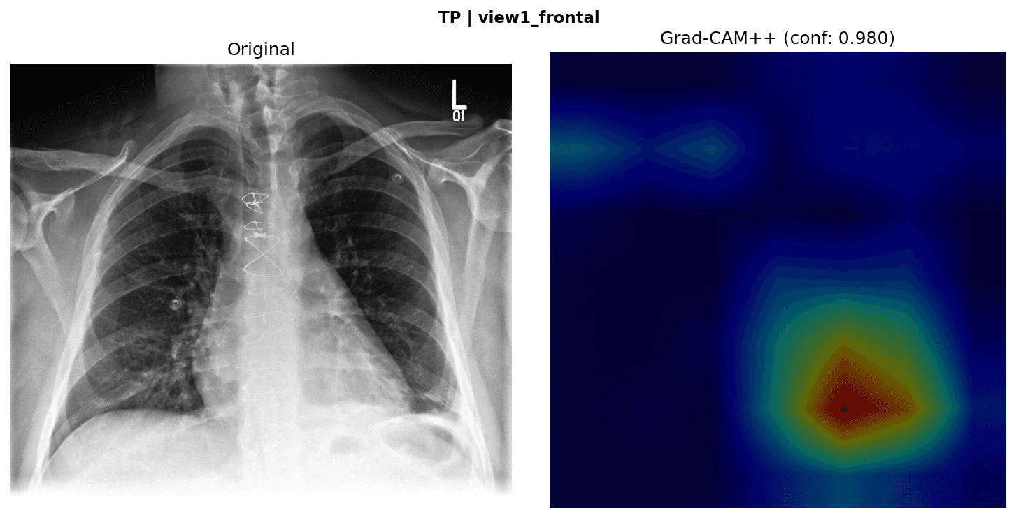
CheXpert has no localisation labels, so I checked the heatmaps visually on 20 held-out test cases (10 true positives and 10 true negatives, picked from the ground-truth labels). The expected pattern for a true positive is concentration at the costophrenic angles in the lower lung fields.
- 20Held-out cases checked10 TP and 10 TN
- 10 / 10TP with lower-field activationLower lung fields and costophrenic angles
- 0 / 10TN with basal concentrationDispersed or in non-diagnostic regions
A failure case: the model that looked at the wrong thing
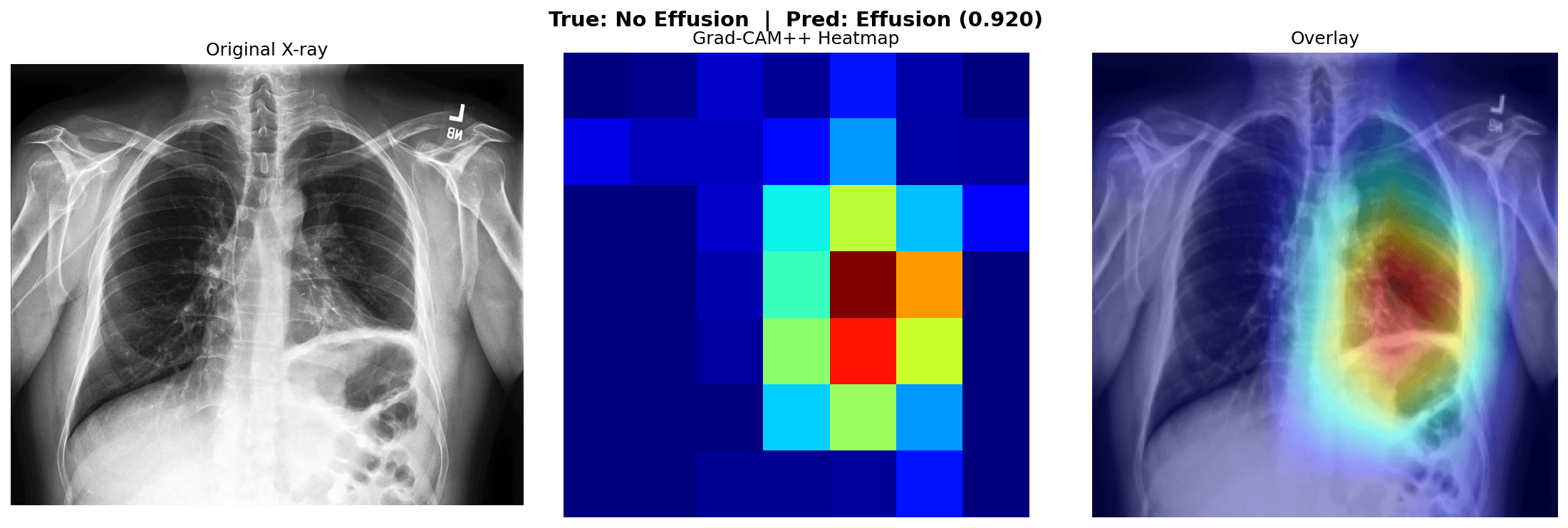
The heatmap shows the prediction was not driven by effusion features at the costophrenic angle. My analysis attributes it to a support device (a line, tube or implanted hardware) in the lower chest: its high-contrast edges produce a strong gradient signal that can dominate the map, which is a known limitation of gradient-based explanations. It is also why the tool's rule is to always read the heatmap alongside the prediction. An unexpected heatmap location is itself a warning about the model's reliability.
Segmentation and the SSM correction
- 164 pxPSPNet lung base (y_max)
- 195 pxSSM-predicted base (y_max)
- 31 pxDisplacement13.8% of image height
- 8%Correction thresholdApplied: yes
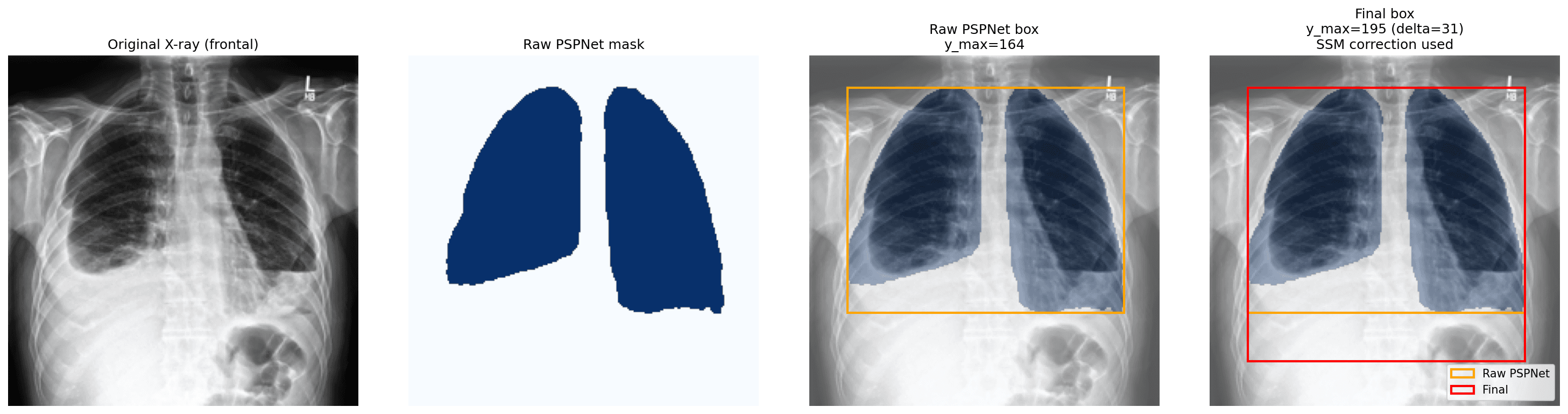
On frontal views PSPNet's mean lung-mask coverage was about 38.5% across 20 validation cases, with both lungs separable every time, and the lateral component filter removed artefact blobs in every tested case. In the corrected example, the Grad-CAM++ peak at y = 178 px would have fallen below PSPNet's boundary (y_max = 164 px) and been clamped to 100% regardless of its true relative position. After correction it is placed inside the lung box.
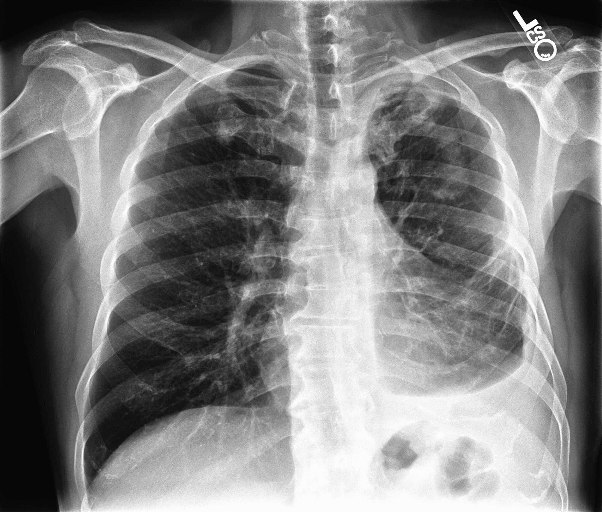
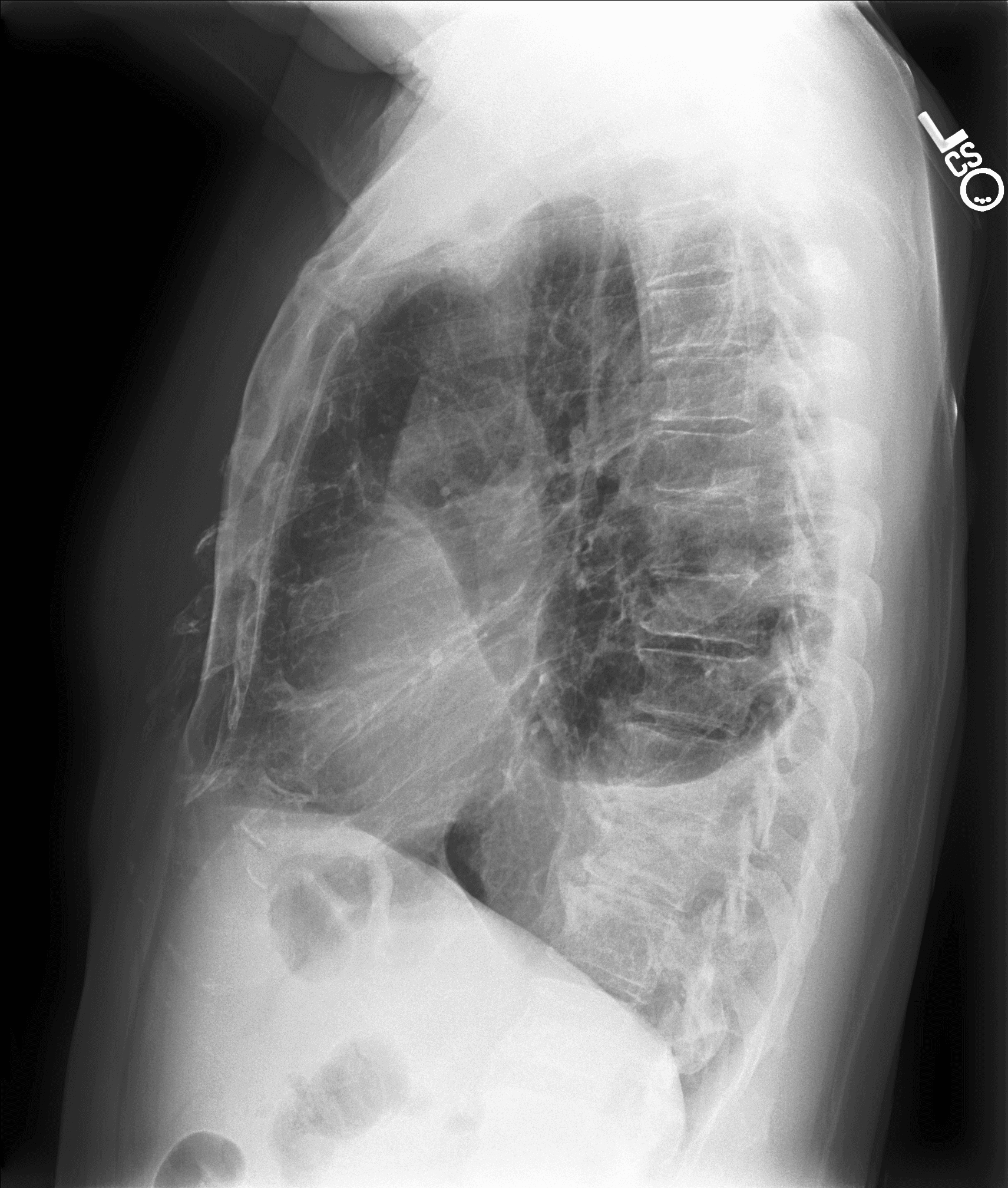
End to end: one patient (CheXpert 00414)
A confirmed effusion case followed through every stage of the pipeline.
1. Input: a frontal and a lateral radiograph
2. Explain: Grad-CAM++ on both views
3. Segment: lung masks
4. Extract coordinates
| Lung | x_pct | y_pct | radius_pct | y_top_pct | y_bot_pct |
|---|---|---|---|---|---|
| Right | 0.345 | 0.975 | 0.167 | 0.778 | 1.000 |
| Left | 0.324 | 0.989 | 0.200 | 0.796 | 1.000 |
Coordinates from the frontal view, as fractions of each lung's SSM-corrected box.
- 0.819z_pct (depth, lateral view)Posterior third of the chest
- 0.597z_extent_pctAnteroposterior length
A y_pct of 0.975 and 0.989 puts both activation centres very near the base of their lungs. A z_pct of 0.819 puts the fluid in the posterior third of the chest, consistent with gravity-dependent pooling in an upright patient. That depth is invisible to a frontal-only system, which would have to place the finding at the middle of the chest.
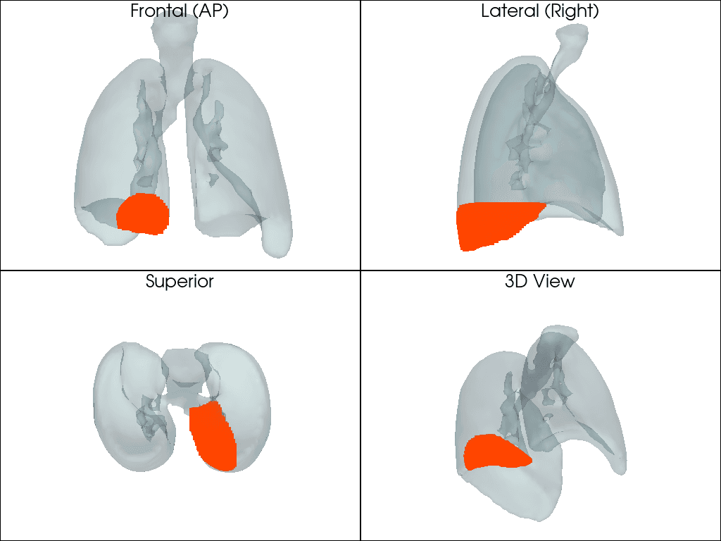
5. Map to the 3D model
| Lung | X (mm) | Y (mm) | Z (mm) |
|---|---|---|---|
| Right | +32.1 | −56 | +163 |
| Left | −40.0 | −56 | +157 |
World positions on the STL model. The model's lowest Z is 156.8 mm, so Z of 157–163 mm is the lung base; Y of about −56 mm sits towards the posterior extent (lowest Y = −82.9 mm).
Three more cases
The same pipeline run on three further confirmed effusion cases. In all three the heatmap activated in the inferior lung regions and the 3D output placed the region at the lung base.
Case 1
Case 2
Case 3
What went wrong, and what I changed
The pipeline went through several redesigns. Each obstacle taught me something about the problem, so I have kept them here.
| Obstacle | What happened | What I did |
|---|---|---|
| Standard image scaling | Near-random predictions | Found that TorchXRayVision expects (x − 128) / 128, and used it for both the classifier and PSPNet |
| Brightness thresholding for lungs | About 93% of the image counted as lung | Moved to deep-learning segmentation: superimposed structures cannot be split by one threshold |
| PSPNet at 224×224 | Noticeably worse masks | Ran it at its native 512×512 and rescaled the boundaries |
| PSPNet on effusion cases | Mask stopped at the fluid line, so the heatmap peak fell outside it | Built the SSM correction, anchored on the reliable upper lung boundary |
| PSPNet on lateral views | Disconnected blobs inflated the depth extent | Kept the two largest components above 500 px² and skipped the SSM |
| Grad-CAM | Risk of one side dominating in bilateral effusion | Switched to Grad-CAM++ after the literature review |
| A single (x, y, z) point | Could not express the size of the effusion | Used a cylinder with radius and anteroposterior extent |
| A floating cylinder in 3D | Would not follow the concave lung surface | Ray-traced a point cloud inside the mesh |
Limitations
- One dataset, one institution. Everything was developed and evaluated on CheXpert. With no cross-dataset test, the accuracy and AUC describe performance inside that distribution only.
- No expert validation of the heatmaps. They were checked visually on 20 cases, with no radiologist review or pixel-level ground truth.
- SSM evidence is thin. It was built from 98 healthy cases and its effect is demonstrated on one case.
- A generic lung. Every patient is mapped onto one average-adult mesh, so the 3D view shows where the effusion sits relative to a generic lung, not the patient's own anatomy.
- The cylinder is an approximation. It looks like a cylinder, not like fluid. A faithful shape would need a learned deformation field or a physical fluid simulation.
- Medical hardware can mislead the heatmap, as the false-positive case shows, so a learner could be misled if they take the overlay at face value.
- More false negatives than false positives, and I did not tune the decision threshold.
- Single pathology, binary output. The model only separates effusion from no effusion.
- Educational use only. CheXpert is a de-identified research dataset and I collected no other patient data. The system is not deployed clinically; any public or patient-facing use would need ethical review and regulatory consideration first.
The code and the full dissertation are private for now.
Where I would take it next
- Radiologist evaluation of a larger sample of heatmaps, and a broader SSM evaluation across effusion severities.
- Patient-specific anatomy. Replace the generic mesh with a CT-derived one where CT exists; the percentage-based mapping could be reused unchanged.
- A more realistic effusion shape, using a physically based fluid simulation or a learned deformation field trained on paired CT and X-ray data.
- A web interface where students upload a paired X-ray and get the classification, overlay, mask and 3D rendering. The backend stages are already modular, so a Flask or FastAPI service would need little adaptation. I scoped it out to keep the focus on validating the core pipeline.
- Multi-pathology output, trained on all CheXpert labels, to show several concurrent findings on the same 3D model.